
|
The basic idea is to consider a population of individuals that each represents a potential solution to a problem. The relative success of each individual on this problem is considered its fitness and is used to selectively reproduce the most fit individuals to produce similar, but not identical, offspring for the next generation. By iterating the process, the population efficiently samples the space of potential individuals and eventually (with probability 1) converges on the most fit solution [Goldberg 89].
Though specific genetic algorithms can be quite varied, all have four essential components:
Strings
Each potential solution to the problem is represented by a string of
values which serves a dual purpose: it provides a representation of what the
solution will become, and it also provides the actual material which can be
transformed (via the operators) to yield new genetic material for the next
generation.
Translation
The process by which strings are translated into possible solutions is
application-dependent and arbitrary. For example, a particular sequence of bits
can be interpreted as a binary-coded number, a Gray-coded number, or a floating
point number by the fitness function. The underlying mechanisms of the GA treat
the same sequence strictly as a syntactic structure independent of translation.
Due to analogies with biology, the string and its corresponding solution are
often referred to as a genotype and phenotype respectively.
Fitness
The environment defines the solution space to be searched. It can be as
simple as a mathematical function, or as complex as a virtual reality where
synthetic animals fight for survival and interact with others of their species.
The environment also provides the mechanism by which possible solutions are
tested. The fitness of the solution refers to how well the solution performs
relative to others in the population.
Genetic Operators
The genetic operators are the methods that transform genetic material of one generation into new and possibly better material in subsequent generations. Most GA's use three relatively simple genetic operators: reproduction, mutation and crossover.
Reproduction
A subset of individuals in the population are selected to reproduce based on their relative fitness values. The reproduction operator simply copies the string from a single parent to child. Used alone, it has the effect of increasing the average performance of the population, but no offspring can be better than their parent.
Mutation
Mutation introduces diversity by randomly changing one or more values in the child's string as shown in Figure 1. Together, reproduction and mutation amount to a random search around the most successful individuals of the previous generation.

|
The crossover operator models sexual recombination. Pairs of strings are chosen as parents. The two strings are cut at a random point along their length then two new strings are created by exchanging the parts as shown in Figure 2.

|
The GA Process
An initial population g0 of N
individuals is generated randomly. Each individual is evaluated by the
environment function which returns a fitness,
 .
The GA then performs two operations. First, the selection algorithm uses the
N fitness measures (one for each individual in the population) to
determine how many offspring each member should contribute to the next
generation. This is often done using the roulette wheel method where
N members are chosen randomly from the population with the
probability of a particular individual being chosen proportional to its
fitness:

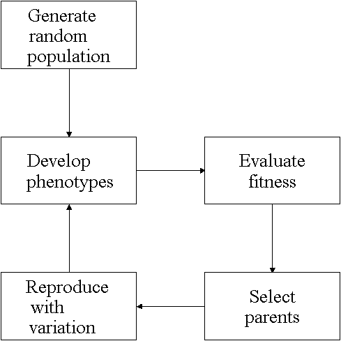
Second, the set of genetic operators is applied to these offspring to make them different from the parents. The resulting population g1 is then evaluated and the cycle repeats itself. The iteration is terminated when the population has converged, a maximum number of generations has been generated, or an acceptable solution is found. A schematic of the process is shown in Figure 3.
|
There are eight major aspects of a PDP model:
Processing Units
All PDP models begin with a set of processing units. In some models, these units represent particular conceptual objects such as features, letters, words, or symbols. In distributed representation models, they are simply abstract elements over which meaningful patterns can be defined.
The number of units is designated N and the units are arbitrarily ordered such that the ith unit is ui. These units do all the processing in the PDP model; there is no executive or other overseer[1].
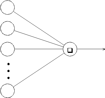
A unit's job is simply to receive input from a set of its neighbors, update its internal state, and compute an output value which it sends to another set of its neighbors (see Figure 4). The system is inherently parallel in that many units carry out their computations simultaneously.
|
The state of the system at time t is usually specified by a vector of N values, a(t), representing the pattern of activation over the set of processing units. The activation of unit ui at time t is designated ai(t).
Output Function
Units interact by sending signals to their neighbors. The strength of their signals is determined by their degree of activation. Associated with each unit, ui is an output function, fi which maps the current state of activation ai(t) to an output signal oi(t):

In some models, the output value is exactly equal to the activation value. More
often,
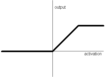
 is some sort of threshold function so that the unit has no effect on its
neighbors until a certain activation value is reached. A threshold function is
displayed in Figure 5.
|
Connection Pattern
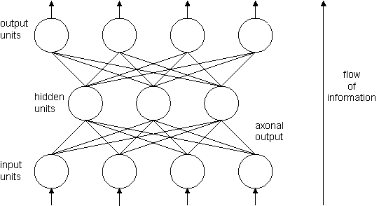
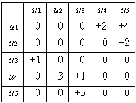
It is the pattern of connectivity between units that determines how the system will respond to a particular input. Perhaps the most well-known artificial neural network architecture is the multi-layer, feedforward network depicted in Figure 6. The units are arranged into layers with every element in a given layer connected to every element at the next higher level.
|
|
Propagation Rule
The rule of propagation takes the output vector o(t) representing the output values of the units and combines it with the connectivity matrix W to produce a net input into the unit:
We also need a rule whereby the net inputs to a particular unit are combined with the current state of the unit to produce a new state of activation. A function F takes the vectors a(t) and net(t) to produce a new activation vector a(t+1). In the simplest case, when F is the identity function, we can write:

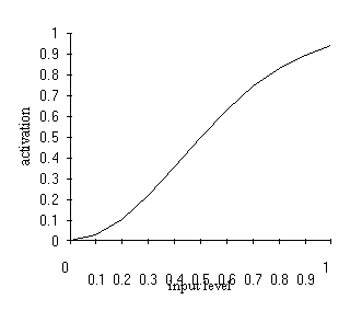
Sometimes F is a threshold function so that the net input must exceed some value before contributing to the new state of activation. The most common class of activation functions is the quasi-linear activation where F is a non-decreasing function of the input:

Figure 8 shows the common sigmoid activation function.
|
Tierra
The Tierran simulator [Ray 92] is a virtual environment that supports the evolution of digital organisms. The organisms themselves are programs written in a specialized machine language. In runs executing billions of instructions, entire ecologies made up of thousands of self-replicating species were seen to evolve.
Organisms
A Tierran creature is a sequence of machine instructions implementing a replicating program. The language was specially designed to be robust under evolution. This was accomplished by two unique features: a truly small instruction set (32 including operands) and a special addressing mode analogous to molecular template matching[2]. Other than these features, the language is typical of most machine languages, consisting of instructions like MOV, PUSH, POP, etc.
Each creature maintains cellular integrity by virtue of the memory services built into the operating system. A creature is allowed to read or execute any memory location, but it is only allowed to write to addresses falling within its own limits. This mechanism has the effect of giving creatures a "semi-permeable membrane".
A creature reproduces by allocating a block of memory adjacent to itself and copying instructions from itself into the new memory. In Tierra, the phenotypes are identical to the genotypes. At the moment of division the daughter creature is given its own virtual CPU. The mother creature is then prevented from writing into the new memory, though it is allowed to allocate a new block.
The World
The Tierran world is a virtual block of RAM known as the "soup". In the original simulations, the soup consisted of 60,000 bytes which held the same number of Tierran machine instructions. At the start of each run, a single hand-crafted self-replicating program is inserted into the soup. Parallelism is simulated by time-slicing: each virtual CPU gets a slice of time on the real CPU as it comes up in the queue.
Eventually all available memory fills up with creatures. This triggers a process called the "Reaper" which kills the creatures. Older creatures and programs which generate more errors while running are more likely to be reclaimed by the Reaper.
Evolution
Variation is introduced into the population with two types of mutation. Bits are randomly selected from the entire soup and flipped at some background rate (typically one bit every 10,000 instructions executed). In addition, bits are randomly flipped during copy instructions.
Mutations alone cannot alter the size of an organism but they can change an instruction so that the creature reproduces incorrectly, creating a daughter that differs in size from itself. Similar mutations inevitably lead to the evolution of a class of creatures called parasites. Parasites cannot reproduce on their own, rather they rely on executing the copying routines of proximal creatures.
The simple evolutionary mechanism of Tierra is complex enough to support an arms race not unlike those between competitive species studied by biologists in nature. In most observed runs the arrival of parasites led to an adaptation in the original population which resulted in a resistance to parasites. The parasites responded with a circumvention to the immunity. Another class known as hyper-parasites evolved which effectively parasitized the parasites.
The Tierra system is available[3] on both UNIX
and DOS and is written in C.
Petworld
Petworld is a simple simulation of artificial animals called pets which eat trees and build nests out of rocks [Coderre 89]. The behavior of a pet is determined by its brain which is a hierarchy of modules called experts. Pet brains are static (i.e. they don't learn from experience) and they are designed, not evolved.
The Petworld system has four major components:
The World
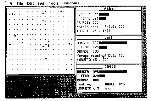
The pets, rocks, and trees of Petworld inhabit a limited two-dimensional Cartesian plane (see Figure 9). Time passes in discrete quanta and simultaneous action is simulated. Pets can travel around in the world, move rocks and eat trees. The trees lose their energy value when they are eaten and regain energy automatically over time (growth).
|
Each pet stores a limited set of variables which indicate the current condition of the animal. Three state variables, hunger, fear, and damage, take on values between 0 and 100. The hunger value is lowered by eating and increases automatically over time. If it reaches 100, the pet dies of starvation. The damage parameter, representing the pet's health, increases when the animal is attacked by another and decreases automatically over time (natural healing). Like hunger, if the damage level reaches 100, the pet dies of its injuries. The fear variable represents how close the pet is to other pets. A low value indicates others are far away while a high value means that another pet is in close proximity. The pet also stores the location of its nest, and a flag indicating whether it is carrying a rock.
Behavior
Pets perform a SEE-THINK-DO loop. Each pet in the simulation is given a chance to perceive its local environment, decide on an action, then execute the action. The decision is made by a pet brain which is programmed by the designer of the simulation. Possible action includes:
Petworld 2.0 runs on an Apple Macintosh and is written in Allegro Common Lisp.
BrainWorks
BrainWorks is an animal construction kit, an interactive computer system that allows novice programmers to assemble active artificial animals out of prefabricated components [Travers 89]. These components include sensors, effectors, computational elements, and structural components such as joints and bones. It also provides a world that supports the co-existence of multiple animals of different species.
The World
The BrainWorks world was designed to be simple, yet complex enough to generate interesting behavioral problems. The world takes the form of a two-dimensional Cartesian plane with objects that exist in a continuous range of positions in contrast to worlds with discrete geometry. It is inhabited by turtles, food, and obstacles. Turtles have zero size, but do have an orientation. Food has no orientation, but has a non-zero radius so turtles can intersect with it. Obstacles are rectangular regions which prevent movement. A scene from the BrainWorks world is depicted in Figure 10.
|
BrainWorks allows the user to construct a nervous system for a simple animal using an interactive graphics editor. The animal is based on the LOGO turtle equipped with eyes, touch bumpers, and motors for movement. The user is supplied with various types of neurons and tools for bringing them into the turtle's body and connecting them to the sensors, motors, and each other.
The computational units are modified McCulloch-Pitts neurons [McCulloch 43] with just two activation states (on or off), and inhibitory or excitatory connections. The set of normal neuron types (input, hidden, output) is augmented by two special types: pulser and delay neurons. The pulser neuron is always activated and can be used to provide default behaviors or to bias other neurons. The delay neuron works like an ordinary interneuron except its output is based on the input values from the previous simulation cycle. Delay neurons can be chained to provide delay lines of arbitrary length. This feature allows the turtle to control the timing of its reactions.
Turtles have three sensors: two eyes and a bumper. The eyes detect food within a conical area of sensitivity controlled by a few internal parameters. The bumper is activated when the turtle hits an obstacle. Movement is controlled by three motor neurons for moving forward, left and right. The magnitudes of movement (linear and angular) are controlled by additional internal parameters. All three may be simultaneously activated, but left and right cancel each other out. A turtle may be wired to display a variety of elementary behaviors such as seeking and avoidance much like Braitenberg's vehicles [Braitenberg 84], but usually its goal is to find food while avoiding obstacles.
Evolution
The BrainWorks system was extended to support reproduction, mutation, and survival contingent on food-gathering performance. Many turtles may compete for limited resources (the food supply) in the world and evolve under the resulting selection pressure.
Survival and reproduction are based on maintaining an energy reserve which is increased by eating and decreased by moving. When a turtle's energy exceeds a certain threshold, it reproduces asexually, passing some portion of its energy to its child.
The neural behavior model was replaced by a matrix representation that mapped the vector of sensory inputs to the vector of motor outputs. When a turtle reproduces, the matrix is mutated by making a small change to one of the elements in the matrix or one of the internal parameters. The two properties of differential survival and reproduction with mutation were sufficient to produce adaptation, however Travers was unsatisfied with the limitations of the system:
Unfortunately the world of BrainWorks is not rich enough to provide a great
variety of possibilities for successful behavior. The turtle can get better at
homing in on food units, and get faster at turning around after striking an
obstacle, but there is not enough room for improvements beyond these. Creating
an artificial world that has enough combinatorial flexibility to permit
innovative behavior is still an unmet challenge. [Travers 89]
Bugland
Bugland is an artificial life world in which the evolving creatures' appearance changes [Rucker 92]. The phenotype reflects genotype, the fitness function is endogenously generated, and genetic algorithm operators are applied automatically.
Organisms
The bugs of Bugland are two and three dimensional Turing machines, and their phenotypes are the trails they leave. The fitness function is generated by having the bugs receive score increments for each trail cell they encounter. The bugs are grouped into colonies and the GA operators are applied within each colony on the basis of the bug's scores.
The behavior of each bug is determined by a set of three lookup tables which are in turn determined by the bug's enzymes and DNA. The enzymes refer to a set of parameters which determine how the DNA is interpreted. A function called DNA_to_RNA uses the enzyme parameters when it translates the DNA bitstring into an appropriate set of lookup tables. This mechanism ensures that every possible DNA bitstring will yield a viable set of lookup tables.
The lookup tables are used for computing the bug's motions, state changes, and output. At each time step the color of the bug's current cell position is read. This input color and the bug's current state are used to lookup the bug's next movement, next state, and an output color.
The World
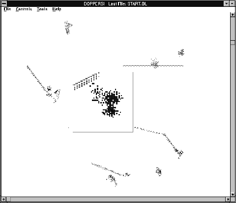
The Bugland world is occupied by one to three separate colonies of bugs. The world can be two- or three-dimensional. In the two-dimensional case, the world takes the form of a discrete lattice with approximately 1000 cells to a side. The edges can be glued together to form a toroidal space or they can be treated as walls which the bugs cannot move across. A screen rendering[4] of the two-dimensional world is depicted in
Figure 11. Cells are colored according to what occupies them. Bugs can distinguish between the following colors: blank, red, green, blue, food, poison, wall, and other. Red, green, and blue are reserved for bug trails, one for each colony.
|
Evolution
A fitness function is modeled by keeping a running score for each bug colony. The score is incremented whenever a bug reads a food cell or a trail cell left by a bug from a prey colony. The score is decremented whenever a bug reads a poison cell or a trail cell left by a bug from a predator colony. The prey-predator relationships and the amounts the score is changed are set interactively by the user.
After a set number of simulation cycles, each colony undergoes breeding. The bugs are ranked from highest to lowest score, and an average score is computed for the colony. Any or all of four kinds of reproduction are then applied to the colony:
1. Sex: the highest-scoring bug is left alone, and the lower scoring bugs are replaced by sexual recombinations of themselves with higher scoring bugs. The crossover operator is applied to the bugs' DNA while the higher scoring bug's enzymes are copied to the child.
2. Mutation: the bug's DNA is randomized. The probability of changing a bit varies from one in ten to one in a million depending on the colony's overall score (higher probability for lower scores and vice versa).
3. Zapping: the worst scoring bug has its DNA completely randomized. This is effectively a 100% mutation.
4. Metazapping: the worst bug has its enzymes completely randomized.
After the breeding, the bugs' scores are reset to zero, and another breed cycle begins.
The latest incarnation of Bugland is called Boppers and runs under Microsoft
Windows. A disk including Boppers comes with [Rucker 93].
P. Computatrix
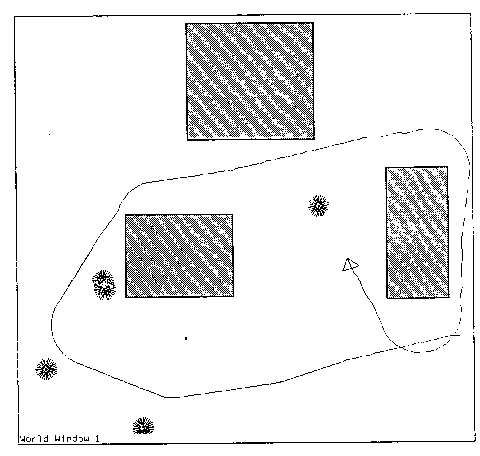
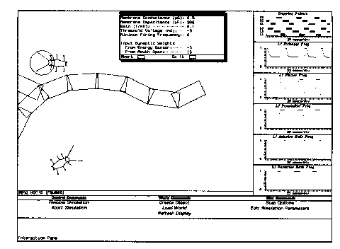
In "Intelligence As Adaptive Behavior", Randall Beer describes the design and implementation of an artificial cockroach [Beer 90]. Complex hexapod locomotion and edge-following behavior were displayed using a network of relatively complex artificial neurons. The insect inhabits a continuous 2-D environment as shown in Figure 12. The network was designed, not evolved.
|
O System
This simulation[5] was designed to evaluate how neural networks undergo change as a result of two forces: learning during the life-time of the network and evolutionary change over the course of several generations [Nolfi 90; Parisi 91]. Organisms consisting of nothing more than the network are simulated foraging for food in a simple two-dimensional grid world.
The World
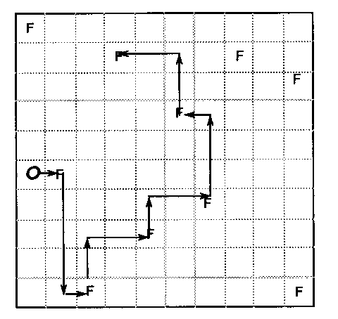
The O System environment is a two-dimensional grid world inhabited by organisms and food units (see Figure 13). An organism (O) or food unit may occupy a single discrete cell. In addition, organisms have one of four orientations. Ten food units are distributed randomly in a 1010 region. Organisms travel around the world and when an O crosses a food unit the food is removed and not replaced. The organism is allowed to move outside the area with food.
|
The behavior of the organism is driven by a simple feedforward neural network with four units in the input layer, seven in the hidden layer, and two in the output layer. Two of the input units are bound to the output units, providing a proprioceptive[6] sense. The other two input units are set to the angle and distance to the nearest food respectively, normalized to a range between 0 and 1. The input layer is fully connected to the hidden layer which is in turn fully connected to the output layer. The output is thresholded to 0 or 1 providing four possible actions:
00 - halt,
01 - turn 90 to the right,
10 - turn 90 to the left,
11 - move forward one cell.
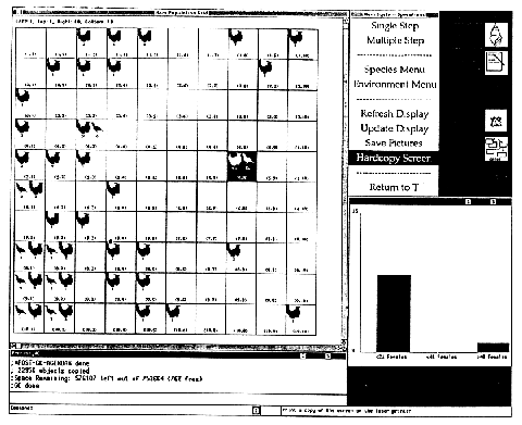
RAM is a simulation shell: it provides time-stepped coordination, a two-dimensional grid space (see Figure 14), the notion of animals-as-processes, graphics and interaction tools, and a consistent set of biological metaphors [Taylor 89]. To construct a biological system within RAM the user must design and program three subsystems: the environment, the species that will populate it, and the observers that gather and display statistics.
Organisms
RAM directly embodies the view that living systems (cells, organisms,
populations) are best understood as processes. It is a step toward addressing
the concerns of those evolutionists who are dissatisfied with these formal
limitations of the current mathematical tools of population genetics
(differential equations, vector fields), and with conceptual limitations of the
non-observable abstractions (fitness functions, selection coefficients) that
one is forced to invent in order to use those tools.
Genesys and AntFarm
Figure 14
Recently, the UCLA Artificial Life group acq
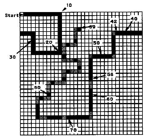
uired a Connection Machine so their current efforts are based on a new systems called Genesys/Tracker [Jefferson 92] (Figure 15) and AntFarm [Collins 92a; Collins 92b]. These systems are not so much toolkits as programs designed to examine the behavior of a particular species, specifically the foraging behavior of ants.
|
PolyWorld
PolyWorld [Yeager 92] is perhaps the most sophisticated of the surveyed systems. It is an ecological simulator that attempts to bring together all the principle components of real living systems into a single artificial living system. These components include biologically motivated genetics, simple simulated physiologies and metabolisms, Hebbian learning in arbitrary neural network architectures, a visual perceptive mechanism, and a suite of primitive behaviors in artificial organisms grounded in an ecology that is just complex enough to foster speciation and inter-species competition. Predation, mimicry, sexual reproduction and communication are all supported in a straightforward fashion.
The World
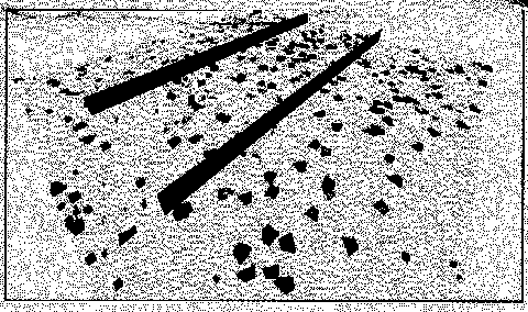
The world is 2-D continuous, and possibly demarcated by a few impassable barriers (see Figure 16). The world is inhabited by freely growing food and a population of organisms. The behavior of each organism is controlled by its neural network. Vision provides the input to the net while the output determines which of a set of primitive behaviors is expressed. Each behavior has an associated energy cost on top of a base cost of living so each organism must forage for food in order to survive. In addition to starvation, the inhabitants have to worry about falling off the edge of the world and defending against attacks from other organisms. The physics of the world is limited to simple collision detection and energy conservation.
|
The organisms have a fixed length genotype consisting of up to a few thousand genes. Each gene is 8 bits in length, representing one of 256 levels between a predefined minimum and maximum value. The first 8 genes control the organism's physiology: size, strength, colour, speed, etc. Interestingly, two genetic algorithm parameters (the mutation rate and number of crossover points) are included in the physiology genes providing a sort of "meta-level genetics" in that the evolutionary process can itself evolve over time.
The remaining genes define the neural architecture using a unique neuronal group representation which greatly reduces the number of genes needed to fully specify an architecture compared to a simpler matrix representation.
Vision
One aspect of PolyWorld that sets it apart from the other simulations is an implementation of a crude vision. A low resolution (2222) image is rendered from each organism's point of view and the resulting pixel map is used as input to its neural net. Only a single row from the image is used for computational efficiency reasons.
Behaviors
The output of the neural net is used to select among a suite of seven primitive behaviors. The behaviors are expressed by raising the activation level of a prespecified neuron over a prespecified threshold. More than one behavior can be expressed simultaneously.
Organisms reproduce by mating. In order to reproduce, two organisms must have overlapping positions and both must express the mating behavior. This method adds a non-random (spatial) element to the genetic algorithm. Whereas most abstract GAs select pairs randomly for reproduction, in PolyWorld organisms only mate with nearby organisms.
Fighting allows one organism to attack another. Like mating, the organisms must overlap, but only one needs to express the behavior. The damage to the victim's health is determined by the attacker's size and strength. If the victim's health goes to zero, it dies and becomes food suitable for eating.
Eating replenishes the organism's internal energy store. The organism's position must overlap some food while it is expressing the eat behavior. The amount eaten is proportional to the activation level.
The organisms travel around the ground plane by expressing the move and turn behaviors. Unless a barrier is encountered, the amount of movement or turning is proportional to the activation of the respective neuron.
An organism can change its field of view by focusing. As discussed in the vision section above, the image representing the organisms view is mapped onto its input neurons. The activation of the focus neuron controls the angle of the field of view.
Finally, lighting refers to changing the brightness of the organism's "face". Since organism's can theoretically see each other, this allows for a primitive form of communication, though none had actually been observed at the time of this writing.
PolyWorld is available[7] on Silicon Graphics platforms and was written in C++.